Amplitude and Phase of a discrete Fourier Spectrum
A. Dieckmann ELSA, Physikalisches Institut der Universität Bonn
![]()
![]()
This tutorial describes the calculation of the amplitude and the phase from DFT spectra with finite sampling. The DFT matrix is intuitively
understood as a set of probes, each sensitive for a certain frequency and corresponding phase information present in a sequential sample of data,
distributed in time or space.
Principle
The multiplication of the complex n × n matrix (there exist several conventions regarding phase and normalization, all working from similar principles...)
![]()
with an array of n real numbers ![]() yields a complex valued vector
yields a complex valued vector ![]()
![]()
that can be interpreted as "Fourier Spectrum". It delivers information about the amplitudes, frequencies and phases of the basic cosines
spanning the function of which an interval having a length of integer number of periods is being sampled into the vector ![]() . The vector
. The vector ![]() consists
consists
of n equally spaced samples, where r is the ‘running’ sample counter. The index r may count samples taken progressing in time or space.
The first sample ![]() corresponds to the value of the sampled function at the left edge
corresponds to the value of the sampled function at the left edge ![]() of the interval
of the interval ![]() and the last sample
and the last sample ![]() is
is
taken at ![]() In this way we get n samples (not n + 1), separated by a distance tt/n.
In this way we get n samples (not n + 1), separated by a distance tt/n.
The complex exponential in the matrix above can be imagined as unit vector that rotates in the complex plane with ‘frequency’ (s-1) / tt and
progressing in time or space ![]() according to the nature of the interval tt. During the matrix multiplication the vector of angular orientation
according to the nature of the interval tt. During the matrix multiplication the vector of angular orientation
corresponding to r is multiplied with the sample of value ![]() and the vector sum is calculated over all r, giving a complex number
and the vector sum is calculated over all r, giving a complex number ![]() . This is repeated
. This is repeated
for all s from 1 to n, each ![]() signaling the presence of a contribution in the samples oscillating with a frequency related to s.
signaling the presence of a contribution in the samples oscillating with a frequency related to s.
The set of all ![]() represents then the spectrum. Note the cancellation of the interval tt inside the argument of the exponential. Depending on the
represents then the spectrum. Note the cancellation of the interval tt inside the argument of the exponential. Depending on the
application ‘spatial’ variables k (wave number) and x (location) or ‘time’ variables f (frequency) and t (time) may be used.
If the samples contain parts changing with the same period as the rotating unit vector this vector sum will exhibit a large magnitude,
because the biggest product vectors all point roughly in the same direction. If the changes of the samples are of a different period with respect to
the rotating unit vector the sums magnitude will be smaller. This will be shown in the next four pictures, their production code is also given.

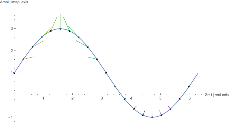
Above we see the rotating unit vector multiplied with a sampled sine function, so the magnitude of the vector is proportional to the
value of the sine. Both are ‘in phase’ (rotation and sine have the same period). The y-t plane of the data and the complex plane of the ‘rotator’
were overlayed. The sine and the vectors appear in the graphic to lie in the same coordinate system and show their relation in a clear way.
The vectors were drawn starting from the position of the sampled points. Negative samples let the rotation phase jump by π.
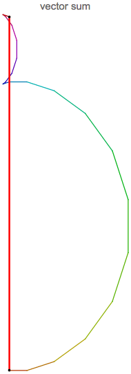
All rotating vectors (complex numbers) are summed and the result (see the red line below, beginning in the origin (0,0) and ending
in the point pe (upper black point)) is large. It corresponds to the Fourier amplitude of frequency 1Hz.

Next the same function is sampled, but the unit vector is rotating more frequently (not once but four times!) within the period of the sine function.
They are ‘out of phase’ and the resulting vector sum will be small.

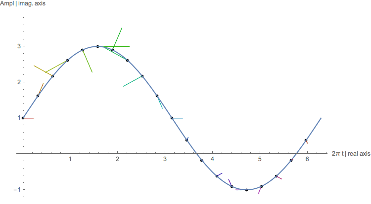
Above we see the rotating unit vector multiplied with a sampled sine function being out of phase (different frequency). The red line
representing the sum of rotating vectors has completely disappeared behind the overlapping black points, see below. The scale is enlarged
compared to the previous vector sum plot (note the length of the edges).

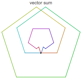
The length of the red line is too close to zero to be displayed :
![]()
![]()
Reconstruction of different Functions from the Fourier Amplitude and Phase
Now we consider more complicated functions. For example let's define a periodic function g[t]

With parameter values given in this example (m = 3) as three triples of amplitude (a), integer frequency (f), phase (φ) and constant ![]()
![]()
and a sampling time interval, that covers a full period interval tt, calculated by 1 / (the greatest common divisor of all contributing frequencies),
![]()
![]()
the function and its cosines look like

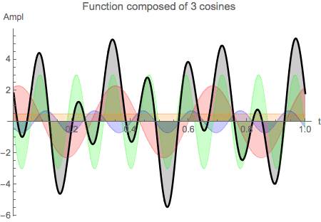
Nyquist's theorem tells us we need at least two samples per period of the highest component frequency ( n > ![]() = 2 tt *
= 2 tt * ![]() ).
).
The lower limit for n lies in this case at
![]()
![]()
and the vector containing the n samples ![]() taken within the interval [tt[ (“closed” to the left, “open” to the right), is calculated. The Drop command
taken within the interval [tt[ (“closed” to the left, “open” to the right), is calculated. The Drop command
is used to get the number of samples right :

![]()
![]()
The next graph shows the function g[t], the samples ![]() and the 'cosine components' of the function
and the 'cosine components' of the function
![]()
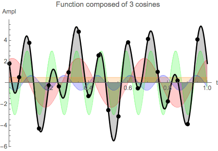
Recall that the first sample sits on the left edge of the interval, whereas the last sample is taken inside the interval near the right edge.
THIS IS IMPORTANT ! Only iff the point on the right edge of the sampling interval of the period is dropped, the correct reconstruction and
periodic continuation is ensured...The reconstructed function will repeat itself outside the interval tt (this is the definition of periodic).
From the samples we get the complex Fourier array
![]()
![]()
and plot the absolute value as spectrum :
![]()
![]()
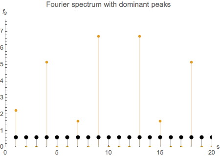
The most relevant bins as well as their mirrors are readily identified (offset in s by 1, because the first term in the spectrum is the one
describing the zero frequency part of the function), all others being zero. Their corresponding frequencies are given by f = (s - 1) / tt in Hertz,
where tt is the full period interval that has been sampled. Apart from the first point the spectrum shows mirror symmetry with respect to
the index ![]() = Ceiling[ (n+1)/2 ], where Ceiling is a function returning the next integer number ≥ its argument.
= Ceiling[ (n+1)/2 ], where Ceiling is a function returning the next integer number ≥ its argument.
Why is the Fourier Array showing a Mirror Symmetry ?
Whenever the phase angle φ of the exponential function in the Fourier matrix would be larger than π, 2π is subtracted and φ stays
in the range -π ≤ φ ≤ π. Instead of counting the phase angle by the left turn it is now (if φ > π) measured by the right turn (in the negative sense of rotation).
This operation leaves the matrix element, which is just a complex number, unchanged. Within the Fourier matrix the phase angle φ increases
with row number reaching the π border at the middle. There will then be pairs of rows with the same (row number) distance to the middle.
The entries of these paired rows will be complex conjugates of each other. So the upper half of the Fourier array, which is a complex vector,
mirrors the lower half with negative phase. In the spectrum plot using absolute numbers we get with increasing s a sequence of amplitude values
up to the highest frequency ![]() , that is visible by the Fourier transformation and that lies in the middle of the frequency indices
, that is visible by the Fourier transformation and that lies in the middle of the frequency indices ![]() = 11 in the above plot).
= 11 in the above plot).
Going further up in s we get the same sequence, but in reverse order.
Finding Amplitude and Phase for select frequencies
The next statement collects all bin numbers of the spectrum with bin values over threshold into a list s. The threshold is used to suppress insignificant bins
(not necessary in this example which is very clean, but add some noise ...) :
![]()
![]()
Now using the Fourier spectrum the offset and amplitudes are found (see next section) to be
![]()
![]()
![]()
![]()
and the phases are
![]()
![]()
from which we can perfectly reconstruct the original function :

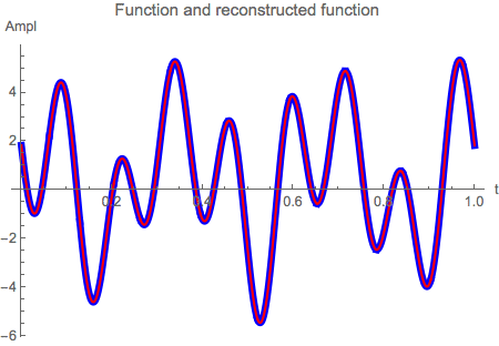
If the original amplitude is negative (in this example a[[3]]), the corresponding phase is offset by π...
![]()
![]()
If a phase lies outside the interval (- π ≤ φ ≤ π) just add or subtract 2 π.
The Connection between Amplitude and Fourier Amplitude
The proportionality factor of the amplitude depends in this normalization convention on the number of samples n.
It can be determined by applying the Fourier transformation explicitly to samples of one simple cosine ![]() + A cos[ 2π f t - φ]:
+ A cos[ 2π f t - φ]:

A look at every frequency s in the spectrum reveals only three non zero entries: The peak in the spectrum lies at s = f + 1 (f ∈ Integers),
its mirror at s = n - f +1 and the zero frequency term at s = 1 :

![]()
The complex number at f + 1 (== Fourier bin) has magnitude A![]() and phase φ. The original amplitude A is therefore obtained
and phase φ. The original amplitude A is therefore obtained
by multiplication of the discrete Fourier amplitude with 2 / ![]() . All other bins in the lower half (s ≠ f + 1) are zero except the
. All other bins in the lower half (s ≠ f + 1) are zero except the
zero frequency term (offset) which comes out as ![]() .
.
Conclusion
Each entry ![]() (s ≠ 1) in the lower half of the Fourier spectrum represents a cosine of frequency corresponding to s with
(s ≠ 1) in the lower half of the Fourier spectrum represents a cosine of frequency corresponding to s with
amplitude ![]() and phase
and phase ![]() being present in the original samples and
being present in the original samples and ![]() is
is ![]() . If there are not enough
. If there are not enough
sample points (Nyquist) or if the interval tt is too short, the analysis gets less precise...The sampled interval is expected to cover exactly
the period of the periodic function. If the function is meant to be non-periodic, ignore the reconstructed part outside the interval.
Additional Example
As an additional example using many more data points consider a function displaying a periodic sequence of pulses defined by edge points:
![]()
This function 'pulse' is sampled within the periodic interval at distances d of the argument x into an array ps with n data points. The increment d
must be small enough to 'grasp the structure' of the pulse (Nyquist theorem...) :
![]()
![]()
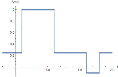
Find the Fourier transformed array :
![]()
The spectrum of the above pulse looks in a logarithmic presentation like

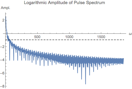
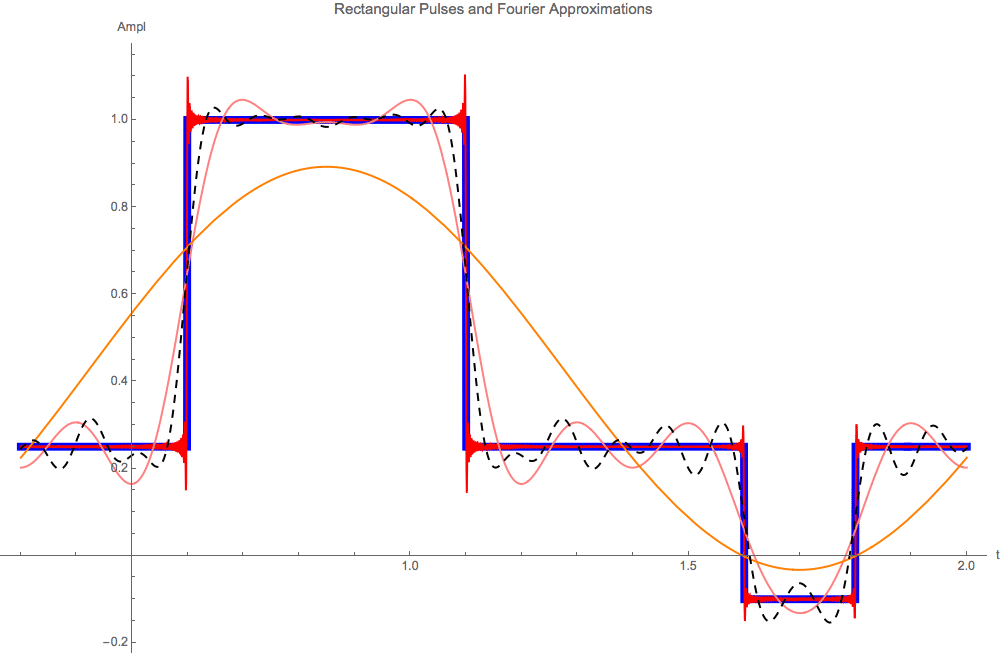
We then get a good reconstruction of the original rectangular pulse function from a superposition of cosine functions with
amplitudes and phases calculated as outlined above using the first half of the (symmetric) Fourier transform array. The first term
represents the 'zero frequency' part, the offset. The frequencies of the contributing cosines are again calculated from their position
in the Fourier array divided by the span of the periodic interval. Also notice the 'Gibbs Phenomenon', the overshoot appearing
at the kinks present in the original function. Shown are different approximations (all terms (red), 9 terms (pink) and 2 terms (orange) of the
Fourier expansion, i.e. different frequency cuts in the spectrum, the black dashed line uses an amplitude cut – only important terms
larger than ampCut are taken into account, the actual position of ampCut in the spectrum is shown in the graphic above with another dashed line.


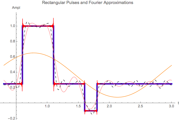
Now with a lengthened sampling interval the period gets longer and the transformation looks differently :

Other Aspects of a Fourier Transformation, Effect of a High Pass
The FourierTransform of a Gaussian pulse is :

![]()
As σ is a positive quantity FourierTransform gives the same result :
![]()
![]()
Plot a pulse:

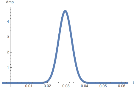
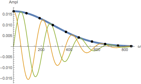
Get the spectrum of amplitudes as the absolute value of the Fourier Transform (as the distribution is again Gaussian
with width 1/σ –> we plot 3 times the width) :

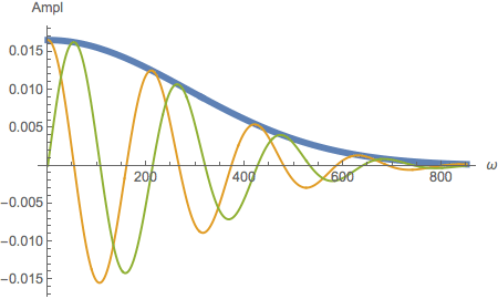
In the plot above also the real and imaginary part of the spectrum is shown, both are formed by a mixture of
frequency dependent amplitude and phase (real part=a(ω) cos(φ(ω)),imaginary part=a(ω) sin(φ(ω))). The value of μ
for example can be found from the period Δω (within frequency space) of real or imaginary part as μ=2π/Δω.
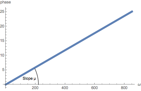
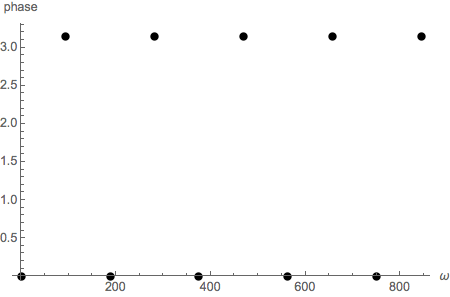
The phase of the Fourier Transform is given by the imaginary part of the argument of the complex exponential divided by the
imaginary unit, it contains the information about the position µ of the pulse given as the slope of the line describing the phase as function of ω :
![]()
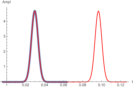
Sample the Gaussian pulse. This function is assumed non periodic, so the sampling interval is chosen such that it covers
the part of the function, that should be analyzed for frequency content or be reconstructed. But the drop of the last sample is still
necessary to get μ and σ - the horizontal scale - right :

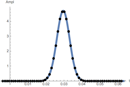
DFT is
![]()
The normalization ![]() makes FourierTransform and Fourier 'equal', jmax corresponds to the 3 sigma width in the Gaussian spectrum :
makes FourierTransform and Fourier 'equal', jmax corresponds to the 3 sigma width in the Gaussian spectrum :
![]()
![]()
The next phase plot shows the same line as in the phase plot above, because - π is equivalent to π (each time the value rises above π,
2π is subtracted...). The Chop on fgs eliminates numerical noise that lets phase values fluctuate from π to -π and backwards.

Plot both reconstructed function and original function, and we see that the DFT continues the original interval as the period of the sampled function :

The red points in the next plot represent the spectrum multiplied with a high pass characteristic, which damps just the amplitude linearly from ![]() to 0
to 0
and leaves the phase untouched :

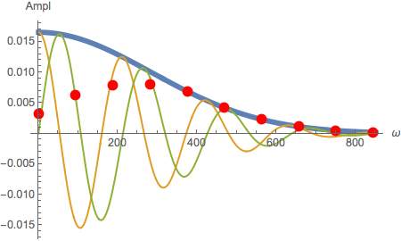
Damp the spectrum at low frequencies:
![]()
The reconstructed pulse (red) shows undershoots :

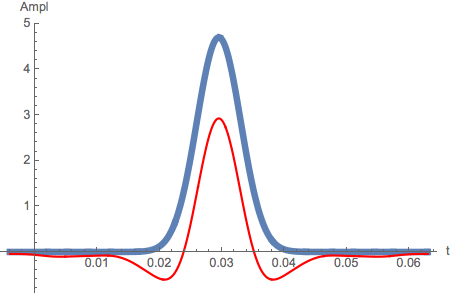
similar for rectangular Pulse, Edge Detection, no low Frequencies
Use same function as above:
![]()
![]()
![]()

Find the transformed array :
![]()
Two basic (complex) transfer functions f(ω) are  (special phase convention by FT in Mathematica...).
This time lets choose the high pass characteristic f(ω) = ω / (ω + i ![]() ) with
) with ![]() = 1 / (R*C) = 333 Hz :
= 1 / (R*C) = 333 Hz :

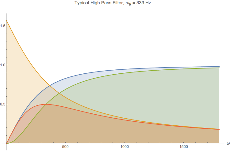
Blue and red show amplitude and phase of the transfer function, green and yellow the real and imaginary part.
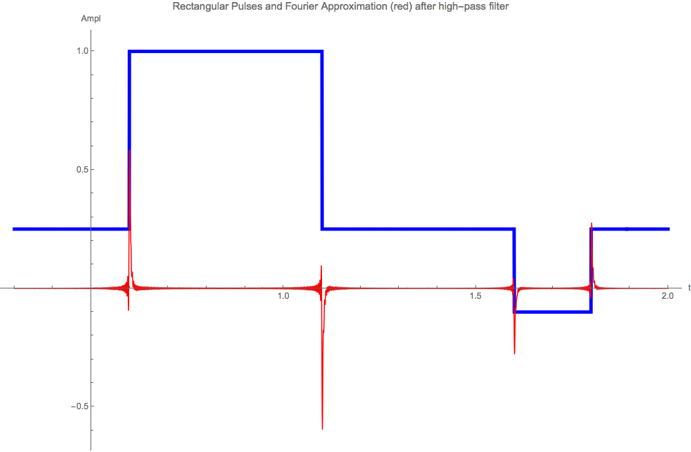
Now we calculate damped spectrum by binwise multiplication of the complex transfer function with the complex Fourier transformed array:


The reconstructed pulse shows mainly the edges of the original, the low frequency part ( ' DC part ' ) is suppressed and change is
emphasized in a differentiated signal:

Afterthought
The point of this tutorial is to demonstrate the working of the Fourier Transform to the newcomer and to show how to avoid certain pitfalls
by giving detailed examples, that may serve as orientation. Good luck!